선형회귀모형 구현실습2
2019-01-28
선형회귀모형 관련 연습문제 풀이
그림, 실습코드 등 학습자료 출처 : https://datascienceschool.net
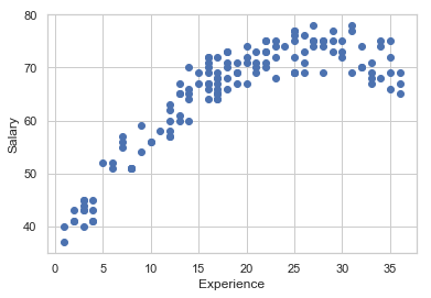
1. 다음은 경력과 연봉간의 관계를 조사한 데이터이다. 차후 나오는 문제들에 대한 풀이를 하시오
# 필요한 패키지 임포트
%matplotlib inline
import numpy as np
import matplotlib as mpl
import matplotlib.pyplot as plt
from patsy import *
# 데이터 로드
df1 = pd.read_csv("http://gattonweb.uky.edu/sheather/book/docs/datasets/profsalary.txt", sep = "\t")
del df1["Case"]
df1.tail()
| Salary | Experience | |
|---|---|---|
| 138 | 43 | 3 |
| 139 | 63 | 12 |
| 140 | 67 | 16 |
| 141 | 71 | 20 |
| 142 | 69 | 31 |
# 데이터 분포 확인
plt.scatter(df1.Experience, df1.Salary)
plt.xlabel('Experience')
plt.ylabel('Salary')
plt.show()
(1) statsmodels를 사용하여 경력에서 연봉을 예측하는 2차 다항회귀모형을 만들어라
sm.OLS.from_formula("Salary ~ Experience + I(Experience**2)", data=df1).fit().summary()
| Dep. Variable: | Salary | R-squared: | 0.925 |
|---|---|---|---|
| Model: | OLS | Adj. R-squared: | 0.924 |
| Method: | Least Squares | F-statistic: | 859.3 |
| Date: | Sat, 19 Jan 2019 | Prob (F-statistic): | 2.43e-79 |
| Time: | 23:17:19 | Log-Likelihood: | -349.51 |
| No. Observations: | 143 | AIC: | 705.0 |
| Df Residuals: | 140 | BIC: | 713.9 |
| Df Model: | 2 | ||
| Covariance Type: | nonrobust |
| coef | std err | t | P>|t| | [0.025 | 0.975] | |
|---|---|---|---|---|---|---|
| Intercept | 34.7205 | 0.829 | 41.896 | 0.000 | 33.082 | 36.359 |
| Experience | 2.8723 | 0.096 | 30.014 | 0.000 | 2.683 | 3.061 |
| I(Experience ** 2) | -0.0533 | 0.002 | -21.526 | 0.000 | -0.058 | -0.048 |
| Omnibus: | 31.087 | Durbin-Watson: | 1.969 |
|---|---|---|---|
| Prob(Omnibus): | 0.000 | Jarque-Bera (JB): | 6.892 |
| Skew: | 0.030 | Prob(JB): | 0.0319 |
| Kurtosis: | 1.926 | Cond. No. | 2.04e+03 |
Warnings:
[1] Standard Errors assume that the covariance matrix of the errors is correctly specified.
[2] The condition number is large, 2.04e+03. This might indicate that there are
strong multicollinearity or other numerical problems.
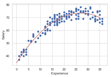
(2) 다음 플롯과 같이 스캐터 플롯 위에 모형의 예측값을 나타내는 코드를 완성하라.
result = sm.OLS.from_formula("Salary ~ Experience + I(Experience**2)", data=df1).fit()
xnew1 = pd.DataFrame(np.linspace(0,35,100),columns=["Experience"])
ypred1 = result.predict(xnew1)
plt.plot(xnew1, ypred1,'r-')
plt.scatter(df1.Experience, df1.Salary)
plt.xlabel("Experience")
plt.ylabel("Salary")
plt.show()
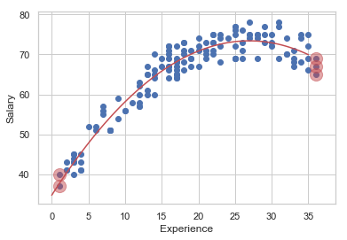
(3) 레버리지가 평균의 3배 이상인 데이터를 찾아서 그림과 같이 스캐터 플롯 위에 표시하여라
influence = result.get_influence()
h = influence.hat_matrix_diag
idx = h > ( 3 * h.mean() )
df1[idx]
| Salary | Experience | |
|---|---|---|
| 21 | 67 | 36 |
| 40 | 65 | 36 |
| 46 | 40 | 1 |
| 60 | 37 | 1 |
| 65 | 69 | 36 |
xnew1 = pd.DataFrame(np.linspace(0,35,100),columns=["Experience"])
ypred1 = result.predict(xnew1)
plt.plot(xnew1, ypred1,'r-')
plt.scatter(df1.Experience, df1.Salary)
plt.scatter(df1.Experience[idx], df1[idx].Salary, s=200, c='r', alpha=0.5)
plt.xlabel("Experience")
plt.ylabel("Salary")
plt.show()
2. 다음은 Defective와 Temperature, Density, Rate 간의 관계를 조사한 데이터이다. 차후 나오는 문제들에 대한 풀이를 하시오
- 종속변수 : Defective
df2 = pd.read_csv("http://gattonweb.uky.edu/sheather/book/docs/datasets/defects.txt", sep = "\t")
del df2["Case"]
df2.tail()
| Temperature | Density | Rate | Defective | |
|---|---|---|---|---|
| 25 | 2.44 | 23.47 | 236.0 | 36.7 |
| 26 | 1.87 | 26.51 | 237.3 | 24.5 |
| 27 | 1.45 | 30.70 | 221.0 | 2.8 |
| 28 | 2.82 | 22.30 | 253.2 | 60.8 |
| 29 | 1.74 | 28.47 | 207.9 | 10.5 |
(1) 이 데이터를 이용하여 선형회귀모형을 구하라
result2 = sm.OLS.from_formula("Defective ~ scale(Temperature) + scale(Density) + scale(Rate)", data=df2).fit()
result2.summary()
| Dep. Variable: | Defective | R-squared: | 0.880 |
|---|---|---|---|
| Model: | OLS | Adj. R-squared: | 0.866 |
| Method: | Least Squares | F-statistic: | 63.36 |
| Date: | Sat, 19 Jan 2019 | Prob (F-statistic): | 4.37e-12 |
| Time: | 23:22:59 | Log-Likelihood: | -99.268 |
| No. Observations: | 30 | AIC: | 206.5 |
| Df Residuals: | 26 | BIC: | 212.1 |
| Df Model: | 3 | ||
| Covariance Type: | nonrobust |
| coef | std err | t | P>|t| | [0.025 | 0.975] | |
|---|---|---|---|---|---|---|
| Intercept | 27.1433 | 1.298 | 20.909 | 0.000 | 24.475 | 29.812 |
| scale(Temperature) | 9.2224 | 4.758 | 1.938 | 0.063 | -0.557 | 19.002 |
| scale(Density) | -6.0354 | 4.945 | -1.221 | 0.233 | -16.199 | 4.129 |
| scale(Rate) | 2.9899 | 3.346 | 0.894 | 0.380 | -3.887 | 9.867 |
| Omnibus: | 2.091 | Durbin-Watson: | 2.213 |
|---|---|---|---|
| Prob(Omnibus): | 0.351 | Jarque-Bera (JB): | 1.491 |
| Skew: | 0.545 | Prob(JB): | 0.474 |
| Kurtosis: | 2.948 | Cond. No. | 8.38 |
Warnings:
[1] Standard Errors assume that the covariance matrix of the errors is correctly specified.
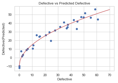
(2) 실제 Defective와 이 모형에서 예측한 Defective 간의 비선형 회귀모형을 구하여 실제 데이터와 회귀 결과를 플롯으로 나타내라. 어떤 비선형 함수를 사용해야 하는가
ypred2 = result2.predict(df2)
df3 = df2.copy()
df3["DefectiveHat"] = ypred2

## np.sqrt => 제곱근(루트) 구하는 함수
model3 = sm.OLS.from_formula("DefectiveHat ~ np.sqrt(Defective)",data = df3)
result3 = model3.fit()
result3.summary()
| Dep. Variable: | DefectiveHat | R-squared: | 0.942 |
|---|---|---|---|
| Model: | OLS | Adj. R-squared: | 0.940 |
| Method: | Least Squares | F-statistic: | 456.3 |
| Date: | Sat, 19 Jan 2019 | Prob (F-statistic): | 7.17e-19 |
| Time: | 23:23:35 | Log-Likelihood: | -86.351 |
| No. Observations: | 30 | AIC: | 176.7 |
| Df Residuals: | 28 | BIC: | 179.5 |
| Df Model: | 1 | ||
| Covariance Type: | nonrobust |
| coef | std err | t | P>|t| | [0.025 | 0.975] | |
|---|---|---|---|---|---|---|
| Intercept | -9.8560 | 1.914 | -5.151 | 0.000 | -13.776 | -5.936 |
| np.sqrt(Defective) | 7.8455 | 0.367 | 21.361 | 0.000 | 7.093 | 8.598 |
| Omnibus: | 0.724 | Durbin-Watson: | 1.684 |
|---|---|---|---|
| Prob(Omnibus): | 0.696 | Jarque-Bera (JB): | 0.600 |
| Skew: | -0.324 | Prob(JB): | 0.741 |
| Kurtosis: | 2.756 | Cond. No. | 12.6 |
Warnings:
[1] Standard Errors assume that the covariance matrix of the errors is correctly specified.
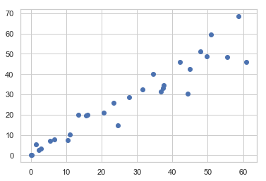
plt.scatter(df3.Defective, df3.DefectiveHat)
xnew3 = pd.DataFrame(np.linspace(0,70,100),columns = ["Defective"])
ypred3 = result3.predict(xnew3)
plt.plot(xnew3, ypred3,'r-')
plt.xlabel("Defective")
plt.ylabel("Defective(Predicted)")
plt.title("Defective vs Predicted Defective")
plt.show()
(3) 위에서 구한 비선형 변환함수를 사용하여 Defective와 예측된 Defective간의 관계를 나타낼 수 있도록 비선형 회귀모형을 만들고 그림을 그려라
model4 = sm.OLS.from_formula("np.sqrt(Defective) ~ scale(Temperature) + scale(Density) + scale(Rate)",data = df3)
result4 = model4.fit()
result4.summary()
| Dep. Variable: | np.sqrt(Defective) | R-squared: | 0.943 |
|---|---|---|---|
| Model: | OLS | Adj. R-squared: | 0.936 |
| Method: | Least Squares | F-statistic: | 143.5 |
| Date: | Sat, 19 Jan 2019 | Prob (F-statistic): | 2.71e-16 |
| Time: | 23:25:52 | Log-Likelihood: | -23.438 |
| No. Observations: | 30 | AIC: | 54.88 |
| Df Residuals: | 26 | BIC: | 60.48 |
| Df Model: | 3 | ||
| Covariance Type: | nonrobust |
| coef | std err | t | P>|t| | [0.025 | 0.975] | |
|---|---|---|---|---|---|---|
| Intercept | 4.7160 | 0.104 | 45.498 | 0.000 | 4.503 | 4.929 |
| scale(Temperature) | 0.8978 | 0.380 | 2.363 | 0.026 | 0.117 | 1.679 |
| scale(Density) | -0.9633 | 0.395 | -2.440 | 0.022 | -1.775 | -0.152 |
| scale(Rate) | 0.3304 | 0.267 | 1.237 | 0.227 | -0.219 | 0.879 |
| Omnibus: | 1.136 | Durbin-Watson: | 1.742 |
|---|---|---|---|
| Prob(Omnibus): | 0.567 | Jarque-Bera (JB): | 0.729 |
| Skew: | 0.380 | Prob(JB): | 0.695 |
| Kurtosis: | 2.935 | Cond. No. | 8.38 |
Warnings:
[1] Standard Errors assume that the covariance matrix of the errors is correctly specified.
ypred4 = result4.predict(df3)
df4 = df3.copy()
df4["DefectiveHat"] = ypred4 ** 2
plt.scatter(df4.Defective, df4.DefectiveHat)
plt.show()